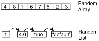
Genetic Operators and Evolutionary Policies

Genetic operators are tools used at each stage of the genetic algorithm. These model the biochemical process that happens at the genetic level. Evolutionary policies are principles enforced during other parts of the genetic algorithm to influence the outcome of the evolution. This section describes a variety of genetic operators that are commonly used, as well as evolutionary policies.

Initialization

When spawning random individuals, it's important to make sure they are as diverse as possible. This means our phenotype-generation mechanism should ideally be capable of creating all legal solutions. The initial population can thereby be representative of the search space. Other genetic operators have this requirement of completeness, too.

Making sure that we can randomly generate any solution is not a particularly difficult task, especially with common genotypes. With more exotic solutions, we'll require some understanding of the data structure used.

Arrays and Lists

Typically, arrays contain a sequence of genes of one data type only (for instance, used to express sequences of actions). Floating-point numbers and single bits are common choices. When initializing such structures, their length must be selected as well as the value of each gene.

Lists are traditionally not restricted to one single data type. They can contain floats, integers, Booleans, and so on. This can certainly be modeled with an array (using one of many programming tricks), but the distinction is historical. Similarly, the length of the list is chosen as well as the values of each gene, but also their type.

Each individual may be somehow constrained. This means the problem requires specific properties from the genotype. For example, an array may need to be a certain length, or the data types in the list may be restricted. In this case, the initialization mechanism should take the constraints into account. This will save valuable time in both the evaluation and the genetic algorithm itself, and improve the quality of the solutions. Figure 32.6 shows a randomly initialized array and list.

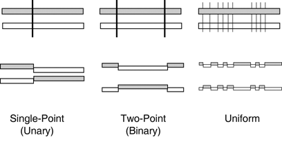
Trees and Graphs

Data structures with higher levels of connectivity prove harder to initialize randomly. A good general-purpose method generates the nodes first, and then connects them together randomly.

For a tree, each node would have one outgoing connection, except the root, which has none. When selecting a neighbor to connect the current node to, the algorithm must not pick one of the descendants (already connected to it). This will ensure that no loops are produced. This will also ensure that the tree is a spanning tree containing all the nodes. To get a binary tree, only parents with fewer than two incoming connections must be chosen.

For graphs, things prove slightly easier. There is no need to prevent cycles because they are allowed—and necessary—in graphs. However, the problem of a single graph spanning all the nodes remains. Sometimes, two subgraphs may be created. If this proves problematic, this case must be identified by a traversal of the data structure. If the graph does not span all the nodes, another random connection can be established. Repeat these steps until the final graph has been built.

Crossover

The genetic operator for crossover is responsible for combining two genotypes. In doing so, a healthy blend of genes from both the father and the mother need to be present in the offspring. This can be problematic, because we want to preserve the good combinations of genes and discard the inappropriate ones. However, it's tough to determine which gene combinations are "fit," so the crossover function needs to be flexible enough to extract these combinations.

Once again, the representation of the genotype is crucial for developing a crossover function. Linear data structures will be able to benefit from biologically inspired crossover techniques, whereas custom designed operators will be needed for data structures with high connectivity.

Regardless of the type of genotype, it's important for the crossover to maintain a consistent data structure; if a specific syntax need to be respected, the operator should not invalidate it. Once again, this will reduce the redundant computation done in the genetic algorithm.

Arrays and Lists

For such linear data structures, a wide range of crossover operations is possible (see Figure 32.7):

• Unary crossover (single point) defines one split point in the parent genotypes. Both are split at this point, and the four parts are permuted and reassembled.

• Binary crossover (two point) instead uses two points to split the parents. This defines a middle segment of the genotype, which is inserted in place of the other parent's segment of genetic code.

• Uniform crossover does not rely on split points. Instead, each gene is randomly copied from either parent. This corresponds to a single split point, but not respecting the order of the genes.

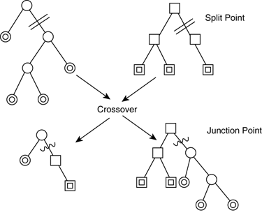
The benefit of each of these operators depends on the meaning of the underlying genome. A fairly safe choice, however, is uniform crossover because it consistently provides a good blend of the genes.

Trees and Graphs

For trees, it's fairly trivial to isolate subtrees and swap the nodes in the genetic code. Doing this once can be sufficient for small trees, but the operation may need to be repeated for larger data structures (see Figure 32.8).

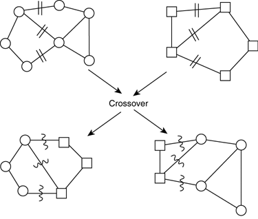
If the trees have well-defined syntax, it's important that the operators check this consistency. (It's often the case here, more so than on lists or arrays.) For each problem, it's important to perform crossover with these constraints in mind.

As for graphs, the issue becomes trickier. Some effort is required to find a good splitting line. First, the set of nodes is divided into two. All the edges that lie within a set (internal) are left intact. The external edges are disconnected and reconnected to random nodes in the other parent genotype (see Figure 32.9).

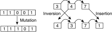
Because keeping all the external edges may lead to dense connections within the graph (O(n²) edges), only half the external edges can be kept. These can be either inbound or outbound edges in directed graphs, or just the mother's or father's edges for undirected graphs.

Mutation

This operator is responsible for mutating the genotype to simulate the errors during fertilization. Such operators generally modify the value of single genes, changing the allele. However, some operations can happen on the genome level, too.

Mutation is responsible for introducing new genetic code into the gene pool, so it's important that this operator be capable of generating any genetic variations. Ideally, the mutation operator should be capable of transforming any genotype into any other—given a sequence of arbitrary transformations. This ensures that the genetic algorithm is capable of exploring the entire search space.

Mutation on single genes is the most common, and applies to almost all data structures. For bits, the mutation can just flip the value. For integers and real numbers, these can be initialized randomly within a range. Another popular approach is to add a small random value to the numbers, as determined by a Gaussian distribution (provided by most random-number generators).

Arrays and Lists

The most common form of mutation happens at the gene level, which is convenient for linear data structures. The mutation operator only needs to know how to generate all the possible alleles for one gene. With a low probability—usually 0.001—the value of a gene should be mutated. Alleles can also be swapped if appropriate.

Given an even lower probability, the length of the data can be changed. The size of arrays can be increased or decreased by a small amount, and list can be similarly mutated. Such operations are done globally, actively changing the size of containers before proceeding. However, a more implicit approach is possible; genes can be inserted or removed from the sequence with an even lower probability. These changes implicitly mutate the length of the genetic code (see Figure 32.10).

This actually can affect the genome itself, which can correspond to meaningless genotypes. Again, if this is the case, the mutation operator should be capable of identifying and preventing this problem. Such structural changes are sometimes not necessary, because the genome is usually well defined and fixed in structure.

Trees and Graphs

For more elaborate data structures, mutation is just as easy on the gene level. Indeed, it's just as easy to mutate an allele if it's a node in a tree, or a graph. These can be swapped also.

In trees, there are also many possible structural mutations. The order or the number of the children can be mutated. Some operators can even swap entire subtrees.

In graphs, structural mutations are trickier. A similar trick can be used as in crossover; the nodes can be split into two groups and reassembled randomly. New nodes can be inserted individually, but it can be beneficial to grow entire cycles at a time. Indeed, in graphs the main difficulty of the evolutionary process is to evolve meaningful cycles.

Selection

The purpose of the selection policy is to decide which parents to pick for breeding, and those that should not reproduce. By using a policy based on the fitness values, elitism can be enforced.

Although each of the genetic operators (that is, crossover, mutate) can be designed to have a beneficial effect on the performance, it's rarely successful and often comes down to educated guessing. On the other hand, the selection policy has a direct influence on the quality of the population—and measurably so.

Fitness Scaling

Before selection occurs, preprocessing of the evaluation results can take place. This may be necessary for multiple reasons [Kreinovich92]:

• The values need to be positive to be interpreted as probabilities.

• The search may be wrongly misled by "super individuals" because of the lack of selective pressure.

• There is no evaluation score per se, because only ranking is possible.

There are some common functions to do this [Goldberg89]:

• Linear scaling uses the function f(x)=ax+b, where the parameters are generally chosen each generation.

• Exponential scaling is based on simulated annealing, where f(x)=e^–bx renormalizes each of the scores given b.

• Ranking associates a fitness for each individual based on their rank, so the result no longer proportional. For example, 1st: 10, 2nd: 9, 3rd: 8, and so on.

This can help iron out the problems with irregular fitness functions to maintain selective pressure on the top individuals. Given the scaled fitness value, different policies can be used in the selection:

• Roulette wheel assigns a slice of the circle proportionally to the fitness. The wheel is spun randomly, and the winning individual gets to mate!

• Tournament selection picks the best from a random group of individuals. One variation involves generating a random number of the magnitude of the fitness, and then picking the highest.

• A ranking policy essentially only allows the top n individuals to mate. This can be done in order.

• Random walk traverses the population stochastically, and picks the best individual encountered. This works well for populations with spatial coherence (for instance, 2D).

• Remainder stochastic sampling allows individuals to mate a number of times , if their fitness is over the average. The remainder of the quotient can be used as a probability to mate again.

Often, fitness corresponds to probabilities for reproduction. These policies provide a way to use the probabilities to create new populations (or parts thereof).

Replacement

This policy varies a lot depending on the nature of the evolution. Generational approaches will not replace any individuals, but rather avoid including them in the next population! On the other hand, replacement is an intrinsic part of steady-state approaches, because room needs to be made for the newest individuals. This section discusses the general techniques used to discard or replace individuals, regardless of the type of population.

It's possible to simulate the generational approach incrementally—potentially using a temporary population—so the steady-state approach can be seen as more generic. When designing the software for this, it may be beneficial to opt for this flexibility.

Two main criteria can be used to replace individuals: fitness and age. However, replacing individuals can be completed by other specific tricks. Common policies include the following:

• If the individual is in the top n%, find another individual at the lower end of the fitness ladder and replace.

• Replace the parents with the offspring (optionally, if the child is less fit).

• Replace the oldest individual in the population with the newest offspring. (This is a hybrid steady-state/generational approach.)

• Individuals found nearby in the population (in 2D grid) can be replaced by local offspring.

These different criteria can combine to estimate the likelihood of an individual being replaced. This value can be interpreted in a similar way to the selection policy (for instance, tournament to determine who dies, and a random walk to find the least fit).